In this tutorial I will show you how to compare two columns in Excel so that the values that appear in both columns become highlighted and you can do something with those duplicate values.
Find duplicate values in two columns
1. Click on the Column Header to highlight Column A.
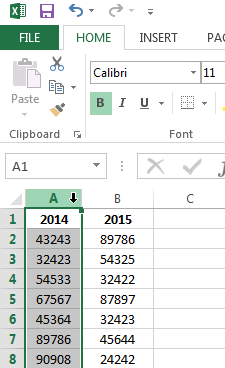
2. Select the Conditional Formatting button on the Home tab.
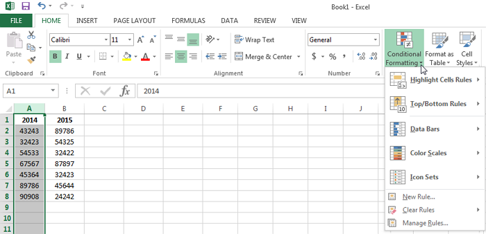
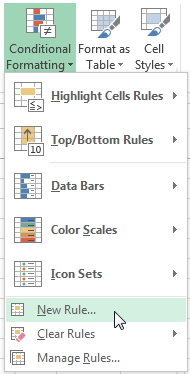
3. Select the New Rule option from the Conditional Formatting button drop-down list.
4. Select ‘Use a formula to determine which cells to format‘ as a rule in the New Formatting Rule window.
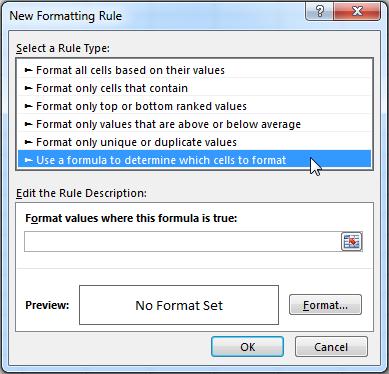
5. Proceed by entering the following formula in the ‘Format values where this formula is true‘ box:
=countif($B:$B, $A1)
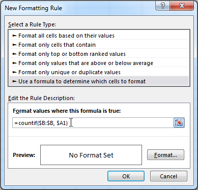
6. Click on the Format button and specify the format you want to set.
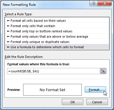
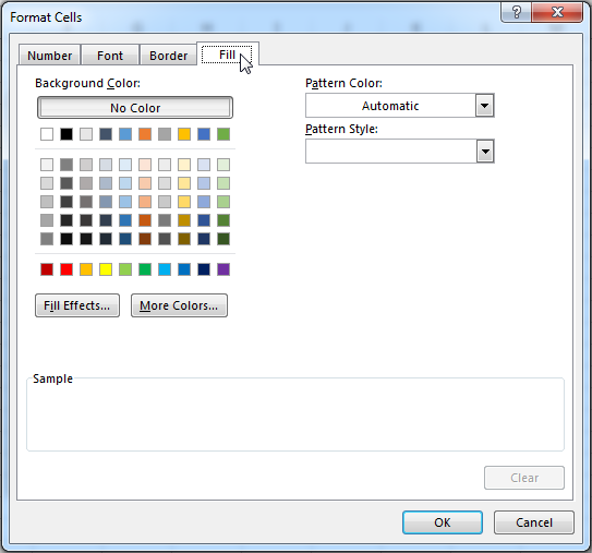
It is possible to set a different cell color for duplicate values by clicking the Fill tab and selecting a background color.
7. After having specified the format you want click OK.
You will be redirected back to the New Formatting Rule window and will be given a preview of the formatting you have selected. If you are happy with the formatting you have specified click OK.
The conditional formatting rule then will be applied to all values of the column and should look like this.
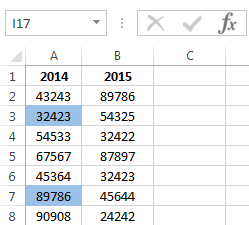
Note how the values of the highlighted cells in Column A are repeated in Column B. I have manually highlighted the cells with identical values in Column B green for demonstrative purposes.
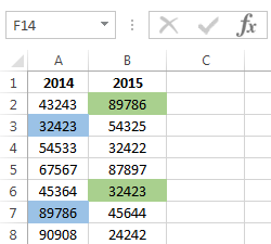
So this is how you can easily see which values are duplicate in different columns in Excel.
Let me know in the comments if I can answer any of your questions!

Hi,
Great Tip. Let us assume we have value 32423 repeated in cell A9, your formula above will also highlight cell A9.
What can I do for cell A9 not to be highlighted.
3. Select the New Rule option from the Conditional Formatting button drop-down list.
Wow, You Rock..
Formula works like a charm..
Thank you very very much..
After following these steps it doesn’t seem to be working in Excel 2010, i get an error message stating that the formula contains an error. I have two columns as well. Column C has 327 entries, column B has 13272 entries. I have to highlight all the matching entries in both columns C and column B.
I nearly admitted defeat, but then I found this. Thank you, from the bottom of my heart!!!
Thanks a lot !!!
SIR HOW TO DETECT SAME TEXT IN ROWS OF TWO DIFFRENT COLUMNS. IF IN ONE COLUMN ONLY TEXT AND IN SECOND COLUMN TEXT WITH NUMBERS OF SYMBOLS.
I’m sure there’s a smarter way to do this, but my first instinct is the follow the following process:
I would split column A into a few different columns. first:
1. insert a few blank columns (3 or so) in between column A & B.
2. Highlight column A, then select “Text to columns” on the data ribbon
3. select “[” as the data delimiter, then select “finish.”
4. Result will be:
Column A: full name, (h.s.c.), EXP, etc. (We’ll fix this in a second)
Column B: 1733-25/09/1995]
5. Insert 4 blank columns between A & B again (to give column A space to split again)
6. “Text to columns” with “comma” as data delimiter, then select “finish”
7. Your result should be:
Column A: Full Name
Column B: (h.s.c.) or applicable
Column C: EXP or applicable
Column D: blank or unnecessary columns, and so on
8. Delete the columns you don’t need, and label the rest accordingly
9. Then, perform your duplicate matching, again, for your “new” full name column.
I hope this helps!
it works perfectly when Column A has more entries the column B or both have same number of entries, but it didn’t work if column A has lesser entries. i don’t know why but it is happening with me in office 2010.
doesn’t work
Mine didn’t work either – only on some duplicates, not all. Wondering if it has to be sorted or something first…
If column A is first names and column B is last names how can I highlight duplicates? I can highlight duplicates in one column but can’t make a rule that only highlights where both columns are equal.
Example, there are 86 Smiths and 41 Alberts. I don’t care to highlight all of those. I do want to see it highlighted if there are 2 Albert Smiths though.
write in column C:
=AND(A1=”Albert”,B1=”Smith”)
This will return TRUE for an albert smith. Then filter the column to only show true values. You can also use advanced conditional formattings too if you know how to use it.
Isn’t that formula only counting the duplicates of the CELL A1 in the entire column B?, what about the rest of cells in A??
I thought that too, so just to be sure, I created another excel to try it out. I put 10 names in column A, and only 4 of them in column B. Column A turned the color I selected in the formatting in the 4 cells that matched what was in column B. I deleted one of the names from column B, and the color went away in column A in the corresponding cell. This was effective. It works either way, A to B, or B to A simply by changing the column letters in the formula.
Thanks bro… it works..
Oh no this is long process, you can do this in simple way there you can find duplicate in both the columns,
1)select both the columns
2)HOME-CONDITIONAL FORMATTING-HI LIGHT CELL RULES-DUPLICATE VALUES.
enjoy GUYS.
This isn’t the same thing. The article talks about when an item in one column matches an item in another column. Your suggestion will simply highlight any cell whose value exists somewhere else in either of the two columns.
That worked perfectly for what I needed…thanks!
Thanks dude you rock!
Thanks Bro…
You’ve really helped me out.
kudos….
super helpful. thanks!
thanks..bro
hi there,
I have a large list with tree names (19000 trees) versus a smaller list (600 trees). I In the large list there are repeats. I want to highlight the tree names in the large list based on all the names fro the small list. This would be the best solution for my taks. When i am using the provided option the cells that contain repeats in the large list (but are not listed in the small one) itself are being highlighted. Can you help on this, please?
In mine, although duplicates in the left hand list are all highlighted, they do also exist in the right hand list. I guess the answer is to strip out duplicates from both lists before you start.
Hi, I am working on a spreadsheet of past sales and we have a lot of duplicates. 5130 lines. Column A is Closing Name (address), Column B is Closed Deal Date, Column C is Actual Sales Price and so on until Column T.
My question is this: Is there any way to merge duplicate lines and have information “win”? Like, If Column A, Lines 6 and 7 are the same, then I want Column I, row 6 to win if row 7 is blank? Does that make sense at all?
Hi,
I want following criteria for my excel it will really helps me if you give me solution for this
In my excel in ‘column A’ I have numbers 1 – 3000 and in ‘columns B’ I am going to enter value randomly between same 1-3000
Now condition: if value in column B matches with Column A it should highlight with colour (eg yellow ) BUT if same value in column B repeated again then it should show error or heigh light with diff. Color (eg Red)
And I want to set this formula for Google sheets :)
Please help me to find out the solution
Thank You Very Much
Please help me further
I need a formula takes unique values of column A(that means no similar values in column A) and highlight the cell it if a unique value exist in column B.
Ex:
A B
11 84
22 56
33 11
44 22
55 22
44 33
66 44
Like in the above example 11 and 33 got highlighted but not 22 and 44.
here I have highlighted font colour but I need cell to be highlighed.
Above formula ” =countif($B:$B, $A1) “”
but it highlights 22 and 44.
I have 2 excel worksheets and I would like to highlight the ones (duplicates) in column A worksheet 1 that are also in column A (or any column) of worksheet 2, I tried vlookup but couldn’t get it to work. can you help?
Thanks for this! Worked really well for what I needed. Unfortunately Excel did decide to freak out when I then tried to filter the data.
Bypassed that problem by turning off the filters, and sorting by cell colour.
I have two columns of data – Column A is name and receipt number, column b is invoice amount. Where column A is the same, I want to review and locate duplicates in column B. I am looking for duplicate postings in the GL under the same customer. Any suggestions?
THANK YOU!
I’m at a total loss after spending hours looking. I have a spreadsheet with Columns A – M.
There are 5097 rows. Several of the rows contain duplicate data across all columns (A-M).
It’s a client list, so from A – M is First Name, Last Name, Address, City, State, Zip, Work Ph, Home Ph, Mobile Ph, Email, Birth Month, Birth Day, Birth Year
I need to find each duplicate row matching across columns A-M and remove them or move them to another sheet.
There are instances where a client is duplicated 8-15 times, but I can’t go through 5097 rows manually and try to remove them.
Thanks so much in advance for any help!
Hi there, How do I run this as a macro?
Your formula is good & helpful . Just I want identical figure coloured on both side automatically. Is there a formula that can colour identical figure both side automatically that I searching for.
Thank a lot it also helpful for me.
Thank you so much, you’ve saved me a lot of time and headache!!!
getting a error – You may not use a reference operators (such as unions, intersections, and ranges) or array constants for Conditional Formatting criteria. What am I doing wrong?
I’ve hightlighted cells in column A that are duplicates of column B using conditional formatting -> =countif($B:$B, $A1). Now if I want to copy those highlighted cells from A into a new column C is there a shortcut for that?
How do I create a formula to search column “A” for X and if found, return the value in column “F”? And possibly, if not found, then leave blank?
This was so helpful! Thank you :D
thank you
Probably this will work for some. Easier for me than inputting formulas. Test it out with typing an real duplicate and you should see the highlighted numbers.
“Example 4. Built-in rule to compare 2 lists and highlight duplicates or uniques
If you are one of those power users who mostly rely on functions and formulas, you may have missed this amazingly simple way to compare two columns in Excel :)
Select two lists you want to compare. If they include different numbers of cells or are located in non-adjacent columns, select the first list, press and hold the Ctrl key, and then select the second list.
On the Home tab, go to Conditional Formatting > Highlight Cells Rules > Duplicate Values.
Select either Duplicate or Unique from the left-hand side drop-down list, and choose the desired format from the right-hand side drop-down. If you are not happy with any of the predefined formats, click Custom format… and set the Font or Fill color to your liking.
Click OK and you are done!”
I have two tables. Table A contains the ID Number and Names of my Staff. This table is from my office database and as a rule, each name begins with the Surname of the staff.
The Staff of recent, went to the bank to open bank accounts. The bank sent me the names and account numbers of the staff in Excel (Table B). However, they did not include the ID Numbers of my staff.
I know that I could easily add the ID Number of the Staff to Table B using the VLOOKUP formula or by creating a query in Microsoft Access that will join the ID number to the names.
However, in this case, I have to first compare the Names in table A to those in table B to ensure that no staff is missing from table B.
The problem I am having is that all the names in the column of names in table A are in this order: Surname-First Name-Middle Name. Some staff use only two names (no middle name) hence, in their case it is Surname-First Name.
However, the names in the column of names in table B are not in any particular order. For some staff, it begins with their First Name and for some, it even begins with their middle name. Only a few actually begin with their surname.
Also, some staff have two names in table A while they have three names in table B and vice versa.
My question is: How can I compare the column of names in table A with that of table B to match the staff in table A that are in table B so that I could afterwards conveniently add the Staff ID to table B?
Thanks a lot. Its quite easy and solved my purpose
Good one..thanks
Quite useful! Thanks a lot. Do you also know how to get the count of these highlighted cells? One thing I can think of is a Sort by Color and manually see till which row number there are colored cells
Very helpful, thanks very much.
Best excel walk thru I’ve come across in a while! Thank you!
Thank you, thank you!
Wish I’d thought to look for this earlier!
Useful, but unfortunately not what I am looking for. How do I compare two separate columns and see if they match?
Edit: https://www.ablebits.com/office-addins-blog/2015/08/26/excel-compare-two-columns-matches-differences/#compare-colums-row-by-row
Dear all. Function not working for me. Can you help?
Thank you!
https://uploads.disquscdn.com/images/eee93f322a74a92241b3f5b4f9d718eec449d9ee4612d2064077b4344b554a68.png
Yeah doesn’t work for me either :(
Try typing countif($B:$B;$A1) instead of countif($B:$B,$A2) . Before $A2, use ; not ,
your recommendation does not solve the error/issue
thanks
thank youuuuuu!!
can we use the conditional formatting for comparing 2 columns. and if cells in both columns have equal value then other column gets highlighted
Hey, very good method.
Do you know how to mark a cell in red in column A, if it is NOT included in the column B? :)
Please help! I have a database with 216 personnel numbers. I exported this to the financial database and use the Vlookup formula to determine how many staff members were paid during the 2017/2018 cycle. I’ve discovered that only 215 people were paid and I now need to determine the missing one to check for reason/s why this employee wasn’t paid. Once I find the personnel number then I can do the investigation as to why this employee wasn’t paid during the cycle.
Does this only work when the two columns are next to each other. I tried this to identify matches from one column in sheet 1 to a column in sheet 2, but it does not work.
Great…How can i move the difference of the 2 colomns to another colomn?
Aha! Thanks
Thank yooouuu!!!
Thank you so much – stopped me making an idiot of myself by writing to same person twice!
Thank you! You made this so easy for me!
Thanks a lot!!!!! It works like a charm!