If you’re used to working in Excel, you’re probably using the SUMIFS, COUNTIFS and AVERAGEIFS functions all the time. When switching to Google Spreadsheet I ran into the problem that I couldn’t use those functions as Google didn’t include them. They only offer the single criterion SUMIF and COUNTIF and don’t support multiple criterion functions. Luckily, they do offer the FILTER function, which we can use to solve this problem. In this post I’ll show you how you can increase your Google Spreadsheet productivity by replicating the behavior of aforementioned Excel functions.
Explaining the FILTER Function
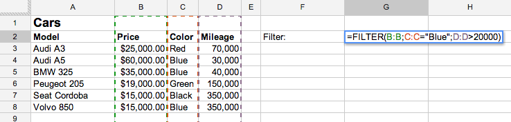
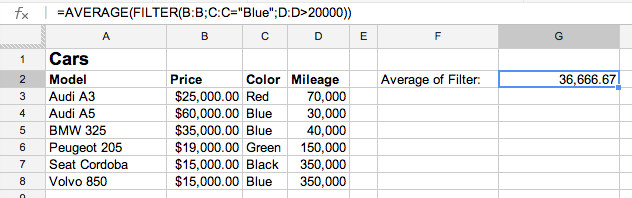
With the FILTER function you can select a range based on one or multiple criteria (up to 30). FILTER(Range; criteria1; criteria2; ...; criteria30) So when you have the following sheet and you want to make a range that selects the price of the Cars that are Blue and that have more than 20.000 mileage you can make the following function: =FILTER(B:B;C:C="Blue";D:D>20000)
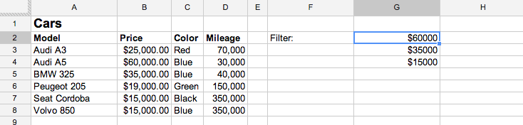
This will return a range with prices of cars that meet your criteria. Understanding this, it’s easy to replicate the SUMIFS, COUNTIFS, and AVERAGIFS functions.
SUMIFS in Google Spreadsheet
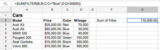
Using the Filter function we now have the prices of all cars that meet our criteria. To sum those prices we can simply use the SUM function on our FILTER Result: =SUM(FILTER(B:B;C:C="Blue";D:D>20000))
And more general: =SUM(FILTER(Range; criteria1; criteria2; ...; criteria30))
COUNTIFS in Google Spreadsheet
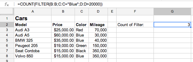
To get the count of cars that meet our criteria, we can simply use the COUNTA function on our filter result: =COUNTA(FILTER(B:B;C:C="Blue";D:D>20000))
And more general: =COUNTA(FILTER(Range; criteria1; criteria2; ...; criteria30))
AVERAGEIFS in Google Spreadsheet
And lastly, to get the average price of the selected cars, we can use the AVERAGE function like this: =AVERAGE(FILTER(B:B;C:C="Blue";D:D>20000))
And more general: =AVERAGE(FILTER(Range; criteria1; criteria2; ...; criteria30))
Note: Google Spreadsheet also doesn’t have the single criterion AVERAGEIF function. You can apply the same method of using the FILTER with only one criterion to simulate the AVERAGEIF function yourself.
That’s it – now you know how to make SUMIFS, COUNTIFS, and AVERAGEIFS in Google Spreadsheet. If you want to see the example in action, check out the following Google Spreadsheet. Let me know in the comments when this tutorial helped you or feel free to ask any questions you might still have!

how do you filter blank cells?
FILTER(A:A;B:B=””) doesn’t work?
I have:
=count(filter(J8:J34, J8:J34″”))
This formula is in J35 and I am not sure if that is effecting it.
I got it too work like this:
=count(filter(A8:A34, A8:A34″”, J8:J34″”))
I had intended to add the other column anyway
Thanks for the blog!!!
Nice solution, great you like the blog! If you want updates on new posts you can subscribe to the newsletter on the right side of the page!
Hi,
your suggestion sounds great, however I am struggling with implementation.
I have google form that is collecting two simple values: child name and status (for example: present or late etc.) Data from the form is saved in google spreadsheet. I am trying to use data from that spreadsheet to prepare summary of how many times particular child was absent present or late.
The problem is that google form is collecting all data in one column, so I have many different names that will repeat down the column. I was trying to filter data according to child name and then use countif to count how many times word “present” occurs. However this is not working at all. Then I found your suggestion. I create the formula but I am getting 0 as the response. Don’t know what can cause such problem. Do you have perhaps any suggestions for what I should look for?
Spreadsheet looks like this: in column b:b are children’s names, in column c:c is their status (so it could be word “present” or “absent”, then i column e:e I have a list of all children and in column f:f I have formula that will count how many times particular words is showing up… looks ok but is not counting according to criteria…
the formula in the cell corresponding to child name is like this: =COUNT(FILTER(B:B=”tom”;C:C=”present”))
Hi Tom, thanks for your elaborate question! I think you can solve the problem using the following formula: =COUNTA(FILTER(B:B;B:B=”tom”;C:C=”present”)).
Note that you start immediately with the criterion, while you have to first give the range you want to select from (B:B). Also because you are counting text, it is better to use COUNTA instead of COUNT. Please see a worked out example I made for you here: https://docs.google.com/spreadsheet/ccc?key=0ApNTZI1iT9tCdE8zSDZsRmJJZjJjTVQzZldnUS15bGc&usp=sharing
Did this help you?
Thank you so much.
Your solution and explanation is brilliant. The formula works great now, and thanks to your explanation I understand now how to use “count” formula. In fact allows me to bring my skills to hole new level ;-)
Thank you one more time!
Glad to have been of help Tom!
If you ever run into other types of questions, don’t hesitate to contact me here or on my email: spreadsheetpro.net [_at_] gmail.com
Hi Tom, Can you set the filter to use an or command? i.e. B=”tom” or “B=”bob”… how would you accomplish the or option? Thank you… Bruce
Please allow me try to answer that question Bruce.
If you go to this example file: https://docs.google.com/spreadsheet/ccc?key=0ApNTZI1iT9tCdE8zSDZsRmJJZjJjTVQzZldnUS15bGc&usp=sharing you can see that you can set another command referring to the value of another cell by simply using B:B=E3 for example (see cell F2 in that file).
Does this answer your question?
Thank you fro taking the time to respond and build a spreadsheet example to explain… that is amazing that you would do that. On your spreadsheet example I’m trying to do something just a little bit different. I’m trying to count the number of times that “Tom” OR “Maria” are “Present” and total in one number. i.e. =Counta(Filter(B:B, B:B=E2 OR B:B=E3,C:C=”Present”)). Is there any way to accomplish that and if so how? Thanking you again. Bruce
If I understand, you only want to filter on whether someone is present? In that case you can leave the name criterion out like this: =Counta(Filter(B:B;C:C=”Present”)). Does this solve your problem?
Thanks for your response again. I’m very sorry, I must not be good at
explaining what I’m trying to do..
What I’m looking for is the OR condition. The filter as is
explained is the AND condition and picks only 1 criteria from each
range, I’m looking for the OR condition which will allow more than one
condition from each range. I did find the answer and the filter works perfectly
in with SUM – for Adding numbers and COUNT – for Counting events.
The formula that I found is (1st is for Adding and 2nd is for Counting)…
=sum(filter(F2:F30; (B2:B30=”Tom”)+(B2:B30=”Maria”); C2:C30=”Present”))
=count(filter(F2:F30; (B2:B30=”Tom”)+(B2:B30=”Maria”); C2:C30=”Present”)).
Notice how the OR condition is structured with the + sign. It uses two conditions with () + () and set as only 1 criteria. Thank you for your interest in helping me solve this problem.
Combining COUNTA and FILTER seems to be working for me for adding multiple criteria to a COUNTIF, but it is returning a 1 in situations when it should be returning a 0. Is there a workaround for this, or do I need a different function?
It indeed does. Here is a solution to mitigate this problem.
You should check first whether a term exist in the target range, and only if it does to the COUNT and FILTER thing.
You can check if some value occurs in a range using this:
=IF(UNIQUE(FILTER(B:B;B:B=E4))=E4,”E4 is in range”,”E4 is not in range”)
Combining this with the COUNT stuff you get for example:
=IF(UNIQUE(FILTER(B:B;B:B=E4))=E4,COUNTA(FILTER(B:B;B:B=E4)),0)
Note that for each extra criterion you want to check it exists, you need to add an extra IF clause with a similar UNIQUE test in your formula.
I followed you until the last part, needing an extra IF clause with a similar UNIQUE test for each criteria. Would you please give me an example of how to test, let’s say, three criteria?
I’m imagining IF clauses within IF clauses, but since I’m not fluent in the UNIQUE function and combining it with the IF confuses me a bit, I’d greatly appreciate an example. Thanks!
I found this, too. It seems to be working, according to my initial tests.
=ArrayFormula(sumproduct(‘Test Results’!B2:B7=”DE”,’Test Results’!C2:C7=”Marketing”,’Test Results’!D2:D7>0))
This works great! Until I try to set a criteria to CONTAINS some text instead of EQUALS some text…
In your example above, this works:
=SUM(FILTER(B:B;C:C=”Blue”;D:D>20000))
but this doesn’t:
=SUM(FILTER(B:B;C:C=”*lue*”;D:D>20000))
The star * should just mark that there can be further text on either side. But adding this star to the criteria seems to break the filter. It doesn’t work for me. Can this be done in other ways?
I’m suffering from this as well. Does anyone know how to make a friggin’ “contains” or “includes” or “like” something that would do this?
=IF(ISNUMBER(FIND(“foo”, D2)), TRUE, FALSE) is what I use to check if a cell (in this case D2) contains or includes the string “foo”. Not sure how to use it in a FILTER, SUMIFS or similar though.
♥
Awesomely simple!
That let me do what I wanted! Here’s how I’ve made my filter:
To have a cell that contains the value of the sum of the cells in column B for the cases in which it’s adjacent cell in column C *starts* with the word “Bank” I did:
=SUM(FILTER(B:B; LEFT(C:C, 4)=”Bank”))
Now with your find, to make that cell sum if it *contains* the word “Bank” it would be:
=SUM(FILTER(B:B; ISNUMBER(FIND(“Bank”,C:C))))
:D
Dear ZippoLag,
I’m trying to use your formula but it’s not working for me :-(
I have this configuration:
– the data to sum in column B.
– the text to be filtered in column E.
I use these formulas:
=sum(filter(B:B;ISNUMBER(FIND(“Asturias”,E:E))))
=sum(filter(B:B;LEFT(E:E, 8)=”Asturias”))
But both shows me “ERROR” and I cannot find the point :-((
Can you please help me out?
Thanks in advance and best regards,
What type of error do you get?
Both of those formulae work for me. So the issue is likely that you have no cells in column E that contain the text string you are trying to find (i.e. “Asturias”).
Help..using the following formula to pull data into another sheet in the same workbook…sheet I am trying to get data from is Philadelphia Inventory and I am trying to count where column H contains 5801 and column B contains scan contract
=COUNTA(FILTER(‘Philadelphia Inventory’B2:B999;’Philadelphia Inventory’H2:H999=”5801″;’Philadelphia Inventory’B2:B999=”Scan Contract”))
Does it work when you change =”5801″ to =5801 ?
No that doesn’t seem to work I get a parse error
Did you manage to get this sorted? i have the same issue…
Thanks
I have the same problem, and am also getting a parse error. My function is: =SUM(FILTER(‘Budget Transfers’!C2:C1000;’Budget Transfers’!A2:A1000=’461000′;’Budget Transfers’!B2:B1000=’330′))
where column A of the Budget Transfers sheet has the ‘461000’ type codes, column 2 has the ‘330’ type codes, and column C has dollar amounts.
This worked great for a simple counting spreadsheet where I was counting up meal totals by table number for my wedding….however do note that if the criteria was not met….(e.g. 0 kids meals at table 5), an unmet criteria will return a value of 1 which might throw things off. Not sure how to prevent this. Thanks for posting though this was very helpful. I don’t get why GD does’t just add countifs
This worked great for a simple counting spreadsheet where I was counting up meal totals by table number for my wedding….however do note that if the criteria was not met….(e.g. 0 kids meals at table 5), an unmet criteria will return a value of 1 which might throw things off. Not sure how to prevent this. Thanks for posting though this was very helpful. I don’t get why GD does’t just add countifs
Thank you!
Since you are article doesn’t offer data to play with (only pictures), I decided to open a spreadsheet for everyone to practice – and improve. I’d be glad if you update your article with the link.
https://docs.google.com/spreadsheet/ccc?key=0ArRQILpPGrQbdFVjUjRhb3BkcHBMakoxVnc1OWtsWFE#gid=0
Hey David,
Thanks for your effort – at the bottom of the article there is already a link to a file for everyone to play with though :)
Cheers,
SpreadsheetPro
Oops, sorry! Well, maybe you should move it to somewhere higher. If I missed it, a lot of people may have missed it too.
Thanks again for this awesome tip!
Dear,
thank you for your help. I’m having an issue that another user report. An unmet criteria will return a value of 1 in stand of 0 which might throw things off (please check my example cell I2)
https://docs.google.com/spreadsheet/ccc?key=0An1f0in9WtyjdEx3X1ZXXzhlbDNLZW9DYmZkaEtOSWc&usp=sharing
Ok, i found out the solution: =counta(iferror(filter(…..)))
Thanks for sharing Fabio!
Hi. I am trying to translate an Excel spreadsheet into a Google Sheet, the lack of COUNTIFS is proving problematic. I have tried using COUNTA(FILTER(…)) but it functions differently to COUNTIFS in a subtle way. In Excel I use COUNTIFS to only count a ‘tick’ if a row above is also ‘ticked’. The COUNTA(FILTER(…)) function doesn’t appear to do that. I wonder if the FILTER(…) function makes a new array that satisfies the conditions and doesn’t check for both conditions to be satisfied relative to each other?
There’s a lot going on with my final equation so I took a screenshot and copied the relevant function into a note available here:
https://www.evernote.com/shard/s100/sh/d01de813-6ac7-4b8b-886a-58d11aff1848/07ff99ce2aecdfd375b8233f84412b29
Maybe this should work and I implemented it badly? Any help would be appreciated.
=sum(FILTER(D:D; B:B=2013; C:C=”Januar”)+FILTER(D:D; B:B=2013; C:C=”Dezember”))
how can i write this simpler?
=sum(FILTER(D:D; B:B=2013; C:C=”Januar” ; C:C=”Dezember”)) Doesnt work, why?
Thanks a lot.
Phil
Phil, it looks like you are using the FILTER() function incorrectly. It filters only one array, whereas you are inputting multiple arrays and attempting to filter according to what is in them. Correct syntax is: FILTER(ARRAY,CONDITION_1,CONDITION_2,CONDITION_3 … CONDITION_30)
Hmm maybe im wrong, but thats how I see it:
This Works just fine:
It should sum all numbers in D if B is says 2013 and C Januar.
=sum(FILTER(D:D; B:B=2013; C:C=”Januar”)
Lets say I have 3 columns:
D = Numbers to be counted
B = Years
C = Months
Now I want to sum all Numbers of the differnt months of 2013.
Like =SUM(FILTER(B:B;C:C=”Blue”;D:D>20000))
But i want =sum(FILTER(D:D; B:B=2013; C:C=”Januar”or”Februar”or”März”…)
The problem is, that my condition “months” are all in the same columns C.
Maybe im totally wrong, but please tell a solution :)
Yeah I’m sorry you were right to reference those other ranges – I deleted my comment after posting it. To be honest I’m not too sure why it isn’t working. I also was having a problem with the FILTER function. Did you see my comment above about COUNTIFS now being included in the new Google Sheets? If you don’t require IMPORTRANGE(), data protection, and a couple of other things right now you could switch to that?
COUNTIFS are included in the new version of Google Spreadsheets:
https://support.google.com/drive/answer/3541068?p=try_new_sheets&rd=1
Thanks Dan! I updated the article to include it.
The formula =COUNTA(FILTER(B:B;C:C=”Blue”;D:D>20000)) worked for me if I use “text” or numbers but I cannot get it to read dates such as: =COUNTA(FILTER(B:B;C:C=”Blue”;D:D12/31/2013))Any ideas will be appreciated.
Thank you very much. That’s exactly what I needed – I used SUM + FILTER combination in my spreadsheet :) It works great and thanks to you I saved a lot of time and my spreadsheet still looks pro ;D
Glad it could help you Mariusz!
no matter what I do with “counta” function…..if my result is “0”, it will always indicate a count of at least “1”. It should give a result of “0”.
anyone solve this?
COUNTA(IFERROR(FILTER(…)))
I need help, in Excel I had the following formula “=SUMPRODUCT((MONTH($G$20:$G$709)=1)*(YEAR($G$20:$G$709)=2013)*($N$20:$N$709))” the goal of this formula is to count all entries in column N that are in January 2013 in column G in a data set containing multiple dates from 2008 to 2014. I cannot get this formula to work in Google Sheets. Can someone help me?
Is there anyway to create if or filter functions for variance or any other functions? I’ve tried =VAR.P(Filter()) and =VAR.P(IF()). Please help make my life easier in my Financial and Environmental Engineering Class!
I am currently using the following formula to count the number of sold units in the last 30 days that matches this criteria.
=ARRAYFORMULA(COUNTIFS(Sold!C:C,”C300W4″, Sold!I:I, “MB CERT”, Sold!B:B,”2011″, Sold!D:D, I7, Sold!AG:AG,”>” &TODAY()-30))
Using the same criteria, I would like to get the average of Sold!AK:AK. How would I do that?
Hi if i want to count both blue and red how can i use?
anybody can help me
=COUNTIF(C7470:C7472,”=red”)+COUNTIF(C7470:C7472,”=blue”)
It will help you
Do you mean if cell background colour is red or blue? If so, that is not possible to do with spreadsheet software. It may be possible to do it with a Google Apps Script in Google Sheets.
I hardly ever leave comments – probably should leave more really – but this was SUPER HELPFUL, thank you so many times.