Excel formatting is changing the way a cell or it’s contents look. There are two ways you can format cells in Excel: you can format the content type of the cell or format the visual look of the cell.
Formatting the cell content
A number for example can be shown as a full number, a number with decimals, a percentage or a currency amount. Dates can be shown in a lot of different ways too.
For this example I’m entering the number 0.4 into cell B2. Click the cell B2, type 0.4 on your keyboard, and press Enter. Excel formats texts that’s entered as general by default.
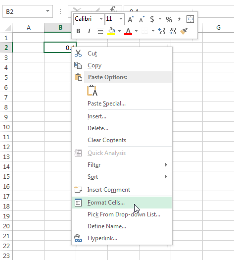
To format a cell’s content as a number simply right-click and choose Format Cells.
Now click OK to confirm the changes to the cell’s format.
In the screen that pops up you see that you can format a cell as different types, or categories.
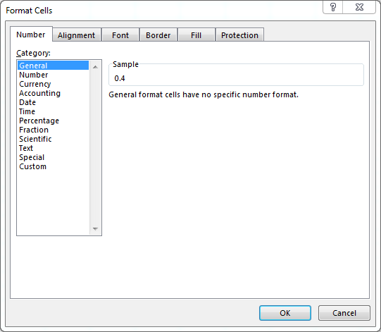
Format a cell as a number
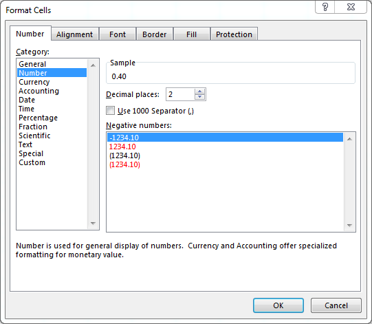
In the popup, click Number to format the cell as a number.
Here you can choose the amount of decimals you want to show and you can toggle whether you want to use a 1000 separator. You can also choose how you want negative numbers to show: with a minus symbol, in red, or with parentheses.
Note that you can see a preview of how your number will look under the Sample section.
Formatting numbers as currency
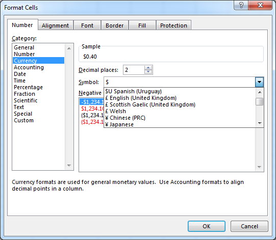
Now select Currency under Category section. Again, you can choose the amount of decimals, but this time you can also choose the currency symbol you want to use.
Formatting numbers as percentage
One other way to will often want to format your cell is as percentage. Click Percentage under Categories and select the amount of decimals.
Please note that originally our number was 0.40 and that it will get multiplied by 100 to show 40%.
Don’t worry, when using this number in calculations, it will still be considered at 0.4.
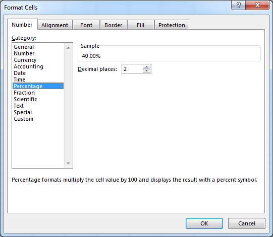
We learned how to format cells as numbers, currency and percentage – these are the most common ones you’ll use. In coming lessons I’ll teach you about other formats, but for now you’re good to go.

Easy way to format cells
As you’ll use Excel more, you’ll start looking for faster ways to do certain actions. As cell formatting is an action you’ll do often, Excel has a quicker way to do it built in into the top ribbon.
Make sure you have selected the Home ribbon and under the Number segment choose the dropdown to quickly format cells in different ways.
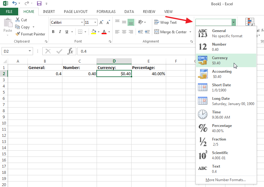
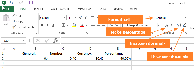
Furthermore, under the dropdown menu you’ll see some extra icons to quickly perform formatting actions.
- The
$sign will let you choose a currency - The
%sign makes your cell a percentage - The other two signs let you increase or decrease the amount of decimals shown in your cell.
Formatting the cell look
So far our spreadsheets have looked quite boring and are all black and white. To change the way your cells look, you can use the Font section under the Home menu in the Excel ribbon on top.
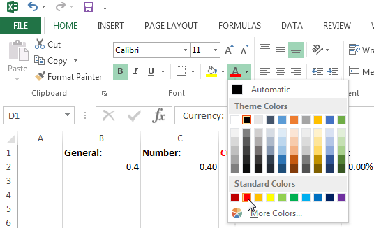
How to change the text color
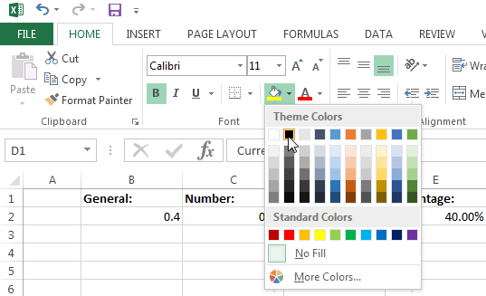
To change the color of the text in a cell click the small icon with A in it and choose your color.
How to change the background color of a cell
To change the background color of a cell, click the Bucket symbol and pick your desired color.
Changing the font, size and look of the text in a cell
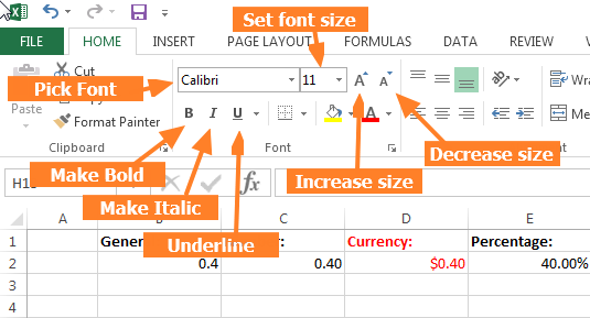
The Font section in the ribbon has a lot of other cool functionalities to manipulate how your text looks. You can:
- Choose a font
- Set the font size
- Increase and decrease the font size
- Make your text bold
- Make your text italic
- Underline your text
Add a border to a cell
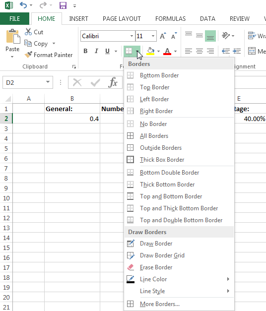
It’s also very easy to add a border to your cells. Simply select a cell or a range of cells and click the border icon in the Font section.
A list of border options will popup. Simply pick where you want to show your border and click.
Change border style and color
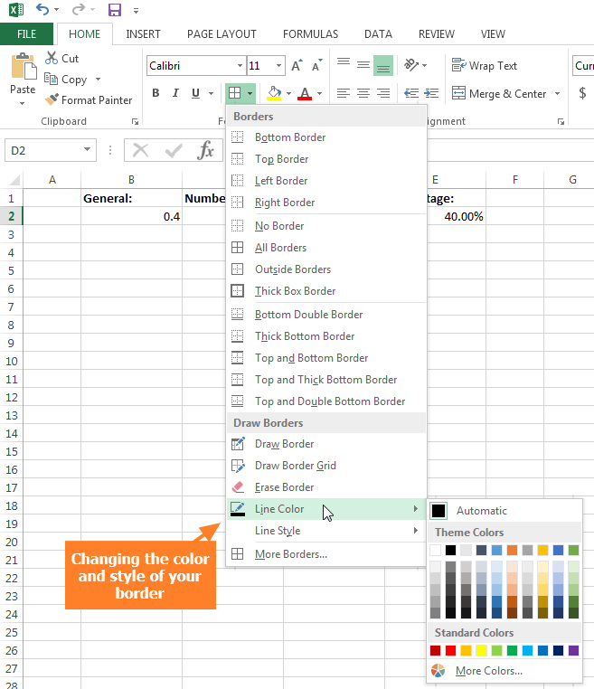
To change the look of your borders to another color click the Border icon again and use the bottom part.
- Select Line color to change the color
- Select Line style to change the style of the border. You can make your border striped in different ways here.
That’s it! There’s a lot more to formatting cells in Excel, but in this lesson I tried to show you the basics. If you want to learn more, check our the other tutorials on SpreadsheetPro.
If you have any questions about formatting, let me know in the comments below!

Speak Your Mind